Introduction
Differential Expression vs Gene Co-Expression Analyses
In transcriptomics, differential expression analysis (DEA) is a standard step to identify genes whose expression levels significantly differ between conditions. This approach highlights candidate genes associated with a phenotype but focuses only on changes in expression magnitude and typically evaluates a limited number of factors or pairwise comparisons. As a result, it does not capture the coordinated behavior or relationships between genes.
Gene co-expression analysis (GCA) complements this approach by focusing on gene interactions. It analyzes expression patterns across all samples to identify groups of genes with similar behavior, known as modules. These modules often reflect shared biological functions or regulatory mechanisms, providing a systems-level view of the data.
While DEA addresses “which genes change?”, GCA answers “which genes work together?”. This distinction is especially relevant in complex experimental designs involving multiple conditions, large sample sizes, or continuous traits, where coordinated gene behavior may not be detected through differential analysis alone.
Among the available methods, Weighted Gene Co-expression Network Analysis (WGCNA) is widely used. It constructs networks based on gene correlations, detects co-expressed modules, and relates them to external traits. This enables the identification of biologically relevant gene groups and potential hub genes for downstream interpretation.
| Aspect | Differential Expression Analysis | Gene Co-Expression Analysis |
|---|---|---|
| Main Goal | Identifies genes that change significantly between conditions | Identifies groups of genes with similar expression patterns across samples |
| Biological question | “Which genes change between conditions?” | “Which genes behave similarly?” |
| Output | A list of differentially expressed genes | Co-expression modules or gene groups |
| What it captures | Expression differences in abundance | Correlation and interaction among genes |
| Best suited for | Simple comparisons such as healthy vs. disease | Complex datasets with many samples, conditions, or traits |
| Interpretation | Useful for finding candidate genes linked to a phenotype | Useful for finding functional groups, pathways, or regulatory modules |
| Main limitation | Often limited to pairwise or few-factor comparisons | Requires sufficient sample structure to detect robust correlations |
Understanding how WGCNA works
Main steps of WGCNA
The analysis starts from an expression matrix (RNA-seq counts) and sample metadata describing experimental conditions or traits. The workflow includes:
- Correlation matrix: compute pairwise gene–gene similarities, typically computed using Pearson correlation.
- Adjacency matrix: transform raw correlations into connection strengths.
- Topological Overlap Matrix (TOM): refine connections between genes by considering shared neighbors.
- Module detection: cluster genes into modules using hierarchical clustering.
This pipeline converts raw expression data into a network where genes are grouped based on coordinated behavior rather than individual expression changes.
Computing gene-gene similarities
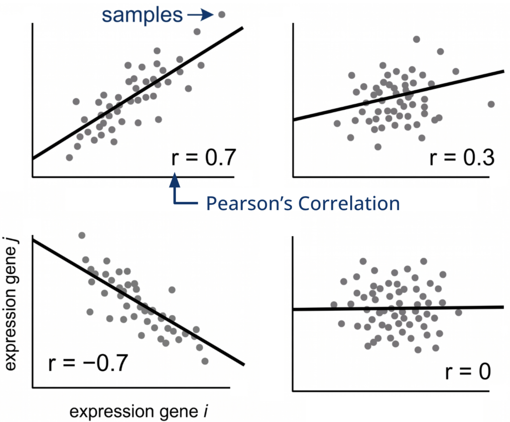
Gene similarity is measured using the Pearson correlation coefficient, which evaluates the linear relationship between expression profiles across samples. Values range from -1 to 1, where positive values indicate co-expression, negative values indicate opposite behavior, and values near zero indicate no relationship.
From correlation to adjacency: why is it needed?
Pearson correlation captures similarity but is not directly suitable for network construction. In co-expression analysis, the focus is on positive relationships; strong negative correlations mean that the genes behave the opposite, so this is treated as “not co-expression”. Thus, raw correlations are transformed into adjacency values ranging from 0 to 1, representing connection strength.
The transformation is performed with the formula 0.5*(1+corr)power , which follows these three steps:
- Shift correlations to a positive range ([0,2]) by adding 1.
- Rescale to [0,1] by multiplying by 0.5.
- Raise the result to a power, which is known as soft thresholding.
Soft thresholding enhances strong correlations and suppresses weak ones in a continuous manner. Higher power values increase this contrast and lead to sparser networks.
| Corr | 1 + corr | 0.5*(1 +corr) | 0.5*(1+corr)6 | 0.5*(1+corr)20 |
|---|---|---|---|---|
| 0.9 | 1.9 | 0.95 | 0.735 | 0.358 |
| 0.5 | 1.5 | 0.75 | 0.177 | 0.00317 |
| 0 | 1 | 0.5 | 0.0156 | 9.53E-07 |
| -0.5 | 0.5 | 0.25 | 0.0002 | 9.094E-13 |
| -0.9 | 0.1 | 0.05 | 1.562E-08 | 1.455E-47 |
How to choose the power for soft thresholding
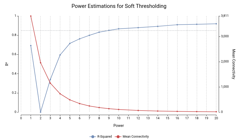
The optimal power is selected to approximate a scale-free topology, a common feature of biological networks, where most genes have few connections and a few genes act as hubs.
The WGCNA package includes a method that evaluates multiple powers and reports the scale-free fit (R²) and mean connectivity. A typical choice is the lowest power where R² ≥ 0.85 while maintaining sufficient connectivity. Lower powers preserve network structure, whereas excessively high values produce overly sparse networks.
Topological Overlap Matrix (TOM)
Adjacency reflects connection strengths between genes but can be sensitive to noise or coincidental patterns. TOM refines these relationships by incorporating shared neighbors. Two genes are considered strongly related if they are directly connected and share similar interaction partners. In biological systems, genes that function together in a pathway usually share a common set of regulatory partners.
This approach reduces spurious associations and better captures biologically meaningful relationships.
Module Detection
Modules are identified by applying hierarchical clustering to the TOM-based dissimilarity. First, the genes are organized into a tree-like structure called a dendrogram, where genes with highly similar connectivity patterns are placed on the same branches.
Modules are then defined using a dynamic tree cut approach, which detects clusters without fixed thresholds. It identifies coherent gene groups, allows further subdivision when appropriate, and assigns unclustered genes to the closest module when possible. More information about the module detection algorithm can be found at Peter Langfelder, et.al. (2009). Finally, each module is assigned a unique color label.
Key WGCNA concepts and terminology
Once modules are identified, several statistics are used to interpret them:
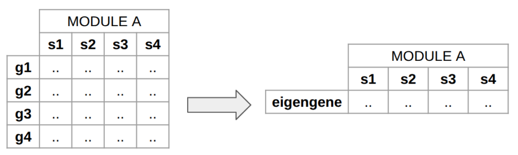
- Module eigengene. It is the first principal component of a module. It represents the overall expression profile of the module. It can be seen as a “summary” of the module.
- Module membership (MM). It quantifies how strongly a gene belongs to a module. It is measured by computing the correlation between a gene and its module eigengene.
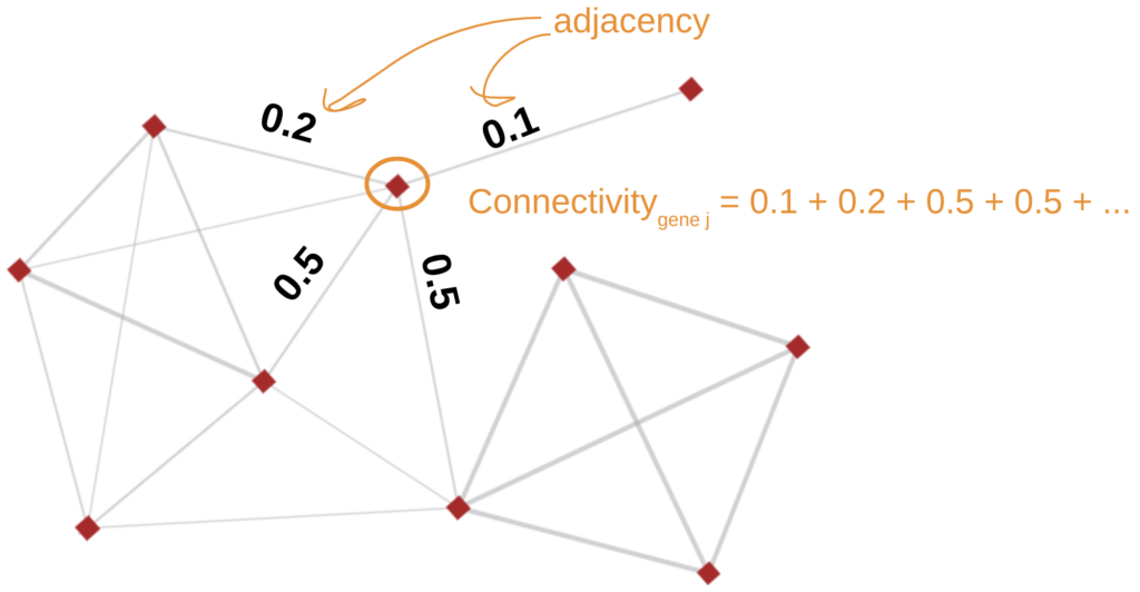
- Intramodular Connectivity. Is the total connection strength (sum of adjacencies) of a gene within its module. Highly connected genes are considered hub genes, often biologically relevant.
- Eigengene–trait relationship. Correlation between experimental conditions (e.g., phenotype, treatment) and module eigengenes. This helps in identifying modules associated with biological traits, enabling the identification of biologically relevant modules.
Gene Co-Expression Analysis in OmicsBox
WGCNA is a powerful but technically demanding method, typically requiring scripting and multiple processing steps. In OmicsBox, this analysis is implemented through a guided and user-friendly interface, enabling its execution without programming expertise.
Configuring the Analysis
The analysis requires gene expression data in the form of a count table, where rows represent genes and columns represent samples. This input can be easily generated within OmicsBox using the RNA-Seq Read Quantification tool, ensuring a complete workflow.
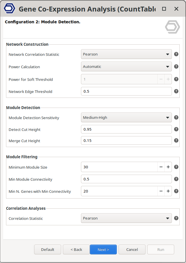
To run the Gene Co-Expression Analysis, the user selects the corresponding option and configures the parameters through a user-friendly interface (Figure 3). Default settings allow a quick start, while analysis parameters can be fine-tuned to adapt the analysis to different datasets. Detailed explanations of the parameters are available directly within the interface by clicking on the question mark buttons, and in the OmicsBox User Manual, facilitating informed parameter selection.
Moreover, all computations are performed in the OmicsCloud, removing the need for local computational resources and enabling the analysis of large datasets.
Exploring the Results
OmicsBox provides interactive and visually rich outputs that simplify result interpretation and exploration (Figure 6).
The main results table summarizes gene-level information, including significance measures and correlations with experimental traits. An additional column includes the module tags, labeled by colors, and an additional “hub” tag. The criteria to identify a gene as a “hub” are configurable. The table columns support sorting and filtering for efficient data exploration.
A set of interactive charts allows rapid assessment of key results, including soft-threshold selection, module–trait relationships, and expression profiles across samples. These visualizations support both quality control and biological interpretation, and are available through the table’s Side Panel with just one click.
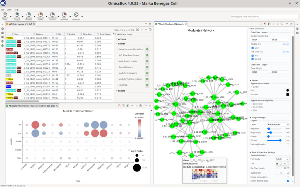
Network visualization is fully integrated, enabling the exploration of modules or selected genes as interaction networks. The interface allows dynamic node filtering, customization of node and edge properties (like color and size), and tooltips including gene heatmaps.
Finally, identified modules can be directly subjected to downstream analyses, such as functional enrichment using Fisher’s Exact Test. This integration facilitates the functional characterization of the biological function of specific gene modules.
Conclusions
Gene co-expression analysis provides a complementary perspective to traditional differential expression approaches by revealing coordinated gene behavior and functional relationships. Through WGCNA, complex transcriptomic datasets can be translated into biologically meaningful modules and key regulatory genes, supporting a deeper understanding of underlying mechanisms.
However, implementing this methodology typically requires advanced scripting and careful parameter tuning. OmicsBox simplifies this process by integrating WGCNA into a guided, interactive environment that simplifies both analysis and interpretation, making it accessible to a broader range of researchers.
Not only the gene co-expression analysis, but the entire workflow from raw RNA-seq reads to gene co-expression analysis can be performed within OmicsBox. This ensures an integrated pipeline where data processing, statistical analysis, and functional interpretation are seamlessly connected within a single platform.
Researchers interested in exploring these capabilities are very welcome to visit the Biobam website and try out how OmicsBox can simplify their analysis by themselves.
About the Author
 Marta Benegas
Marta studied biotechnology at the Valencia Polytechnic University (UPV) and continued her studies with a Master's in Bioinformatics at the Autonomous University of Barcelona (UAB), Spain. After her master's degree, she started her professional career at Biobam where she is now working as a bioinformatics specialist and support manager. At the moment she is mainly focused on Single-Cell technologies developing various pipelines which allow getting from reads to functional insights at a single-cell resolution. These developments are available in OmicsBox, BioBam’s software solution.