Single-cell RNA-Seq (scRNA-Seq) analysis has been widely used to investigate animal tissue heterogeneity, principally with human and mouse data. However, this technique is increasingly being used to study plant tissues as well with comparable results. Despite the challenges it faces due to the plant cell wall, researchers have been able to perform single-cell analysis with plant protoplasts, bringing the power and granularity of scRNA-Seq analysis to the plant kingdom.
In this blog, we will reproduce the analysis performed by Shulse et al., 2019 and study the root of Arabidopsis thaliana at the single-cell level using OmicsBox. In this study, the researchers used Drop-seq to obtain scRNA-Seq data from A. thaliana roots grown in normal and high-sucrose mediums. They sequenced multiple root samples and identified the different cell types present in this tissue, as well as the differences in both the abundance of cell types and gene expression between the different grown conditions. We will go through the entire scRNA-Seq analysis pipeline, starting from raw reads down to functional insights. We will go through each step thoroughly and give some advice for successful analysis, hoping this blog serves as a guide for single-cell transcriptomics analysis.
Data
- Raw sequencing data is available in the NCBI GEO database with accession GSE122687.
- 10 samples of Arabidopsis thaliana roots from 7 different seedlings were sequenced (named Replicate A to J).
- 3 samples were grown in a high-sucrose medium and 7 in a normal medium.
- Single-cell RNA-Seq libraries were obtained with Drop-seq version 3.1.
- The sequencing was performed with Illumina NextSeq 500 (7 samples), Illumina HiSeq 4000 (2 samples), and Illumina HiSeq 2500 (1 sample).
scRNA-Seq Analysis
FASTQ Quality Check
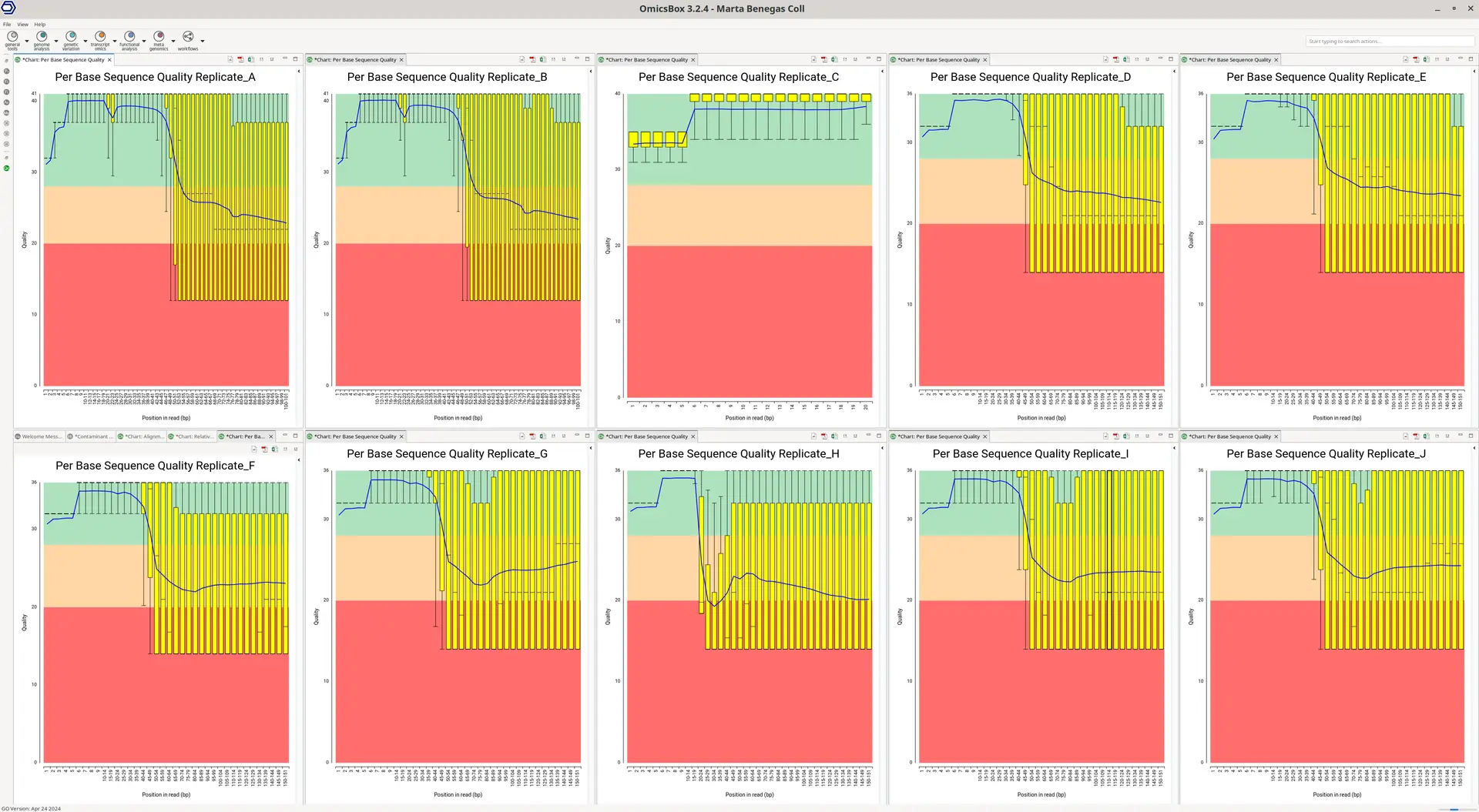
Even when downloading sequences from GEO, it is good practice to perform a FASTQ Quality Check and check the quality and characteristics of the data.
For this particular dataset, we saw a sharp drop in the quality of the upstream reads after the first bases in almost all samples (Figure 1). In libraries constructed with the Drop-seq technologies, the first bases of the upstream reads contain a Cell Barcode and a UMI, short sequences to identify the reads belonging to a particular cell and transcript, respectively. The rest of the upstream and the downstream reads contain actual cDNA (or transcript) sequences.
Due to the per-base sequence quality for each sample, we decided not to use the cDNA sequence of the upstream reads for alignment and quantification, even though it is generally recommended to use them if available.
scRNA-Seq Quantification
Reads were aligned to the reference genome and quantified with the STARsolo implementation in OmicsBox, which allows a highly customizable quantification. In order to keep a higher number of alignments for quantification, we configured the analysis to keep both reads aligning to exonic and intronic regions, as well as multi-mapping reads. To decide the gene to assign a given count, we used the “Rescue” strategy. This method distributes the counts uniformly among the multi-mapping UMIs in a way proportionally to the sum of uniquely mapped UMIs (Mortazavi, A., et al.,2008).
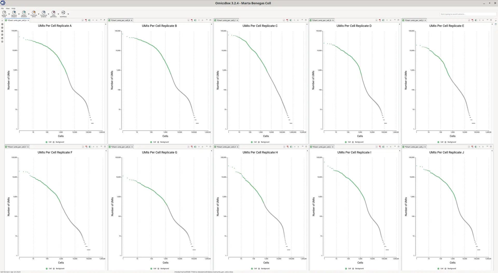
Aside from the count matrix, a Barcode Rank Plot is generated (Figure 2), which helps assess if the number of detected barcodes (cells) in the dataset is correct. On the X-axis, cells are ordered by the total number of UMIs (transcripts) detected, which is displayed on the Y-axis. For droplet-based technologies, it is common to see a harsh drop on the plot. After this area, the detected barcodes are considered to be background noise, contaminant mRNA, or sequencing errors.
This plot shows in green the barcodes that have been kept, and thus considered to belong to actual cells. In this case, we considered that the number of cells kept was correct since the green-colored cells end in the middle or before the sharp drop. Additionally, the overall alignment rate was good (ranging from 50% to 80% of aligned reads), with a mean UMIs per cell of 4500.
💡 How to handle multiple-sample scenarios
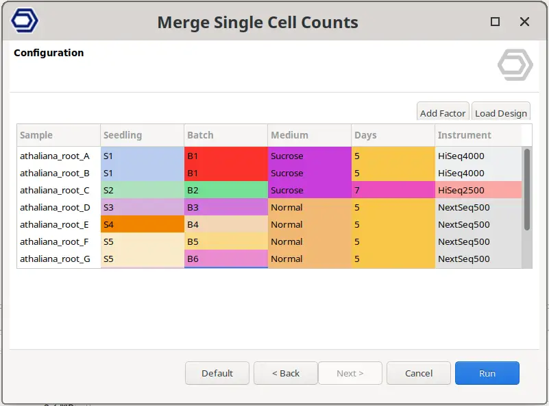
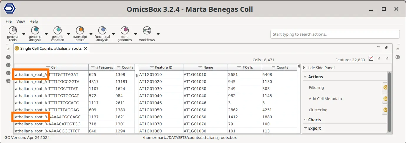
It is important to note that, since the Cell Barcodes can be repeated in different sample preparations, the quantification has to be performed for each sample separately. Then, in order to analyze all samples together, we first need to join the count tables. This can be achieved with the Merge Single Cell Counts tool in OmicsBox. This tool allows specifying the experimental design effortlessly (Figure 3), since the factors specified for each sample will be applied to all its cells. Moreover, this tool automatically adds a suffix to each cell barcode so they are unique (Figure 4).
Cell and Gene Filtering
Both cell and gene filtering were performed using the Single-cell RNA-Seq Filtering tool in OmicsBox, which makes use of the Seurat R package.
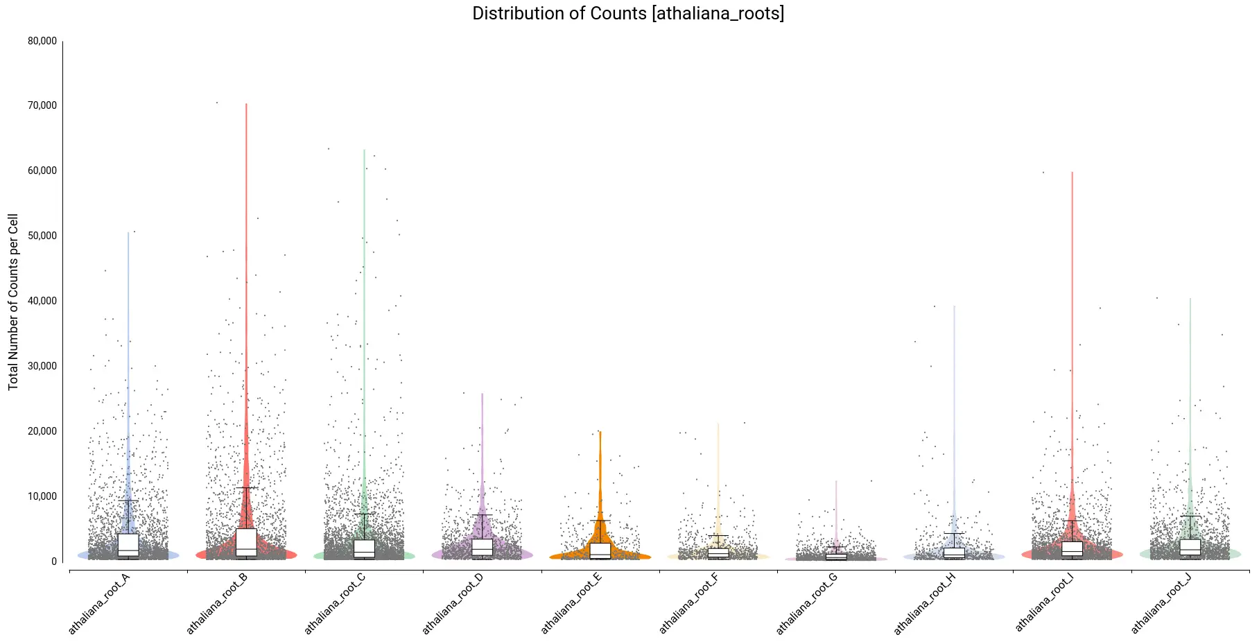
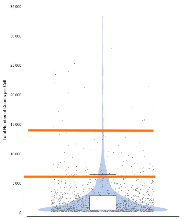
To decide filtering thresholds, violin plots were generated with OmicsBox in order to assess the per-cell counts distribution for each sample (Figure 5). These plots allow easy identification of the outlier cells, both with a comparatively higher amount of total counts (that could correspond to doublets or multiplets) or with a comparatively lower amount of total counts (that could introduce noise to the downstream analysis).
In addition, box plots are shown on the top of the violin, which gives a more precise description of the distribution with statistical values such as Q1, median, Q3, etc.
For this particular dataset, all samples have a minimum number of total counts per cell of 370 or higher, so we decided not to put a minimum filtering. This is probably because the STARsolo tool used for quantification already filters cells with a small number of counts, since they may not be detected as truly cells. Open image-20240510-100423.png
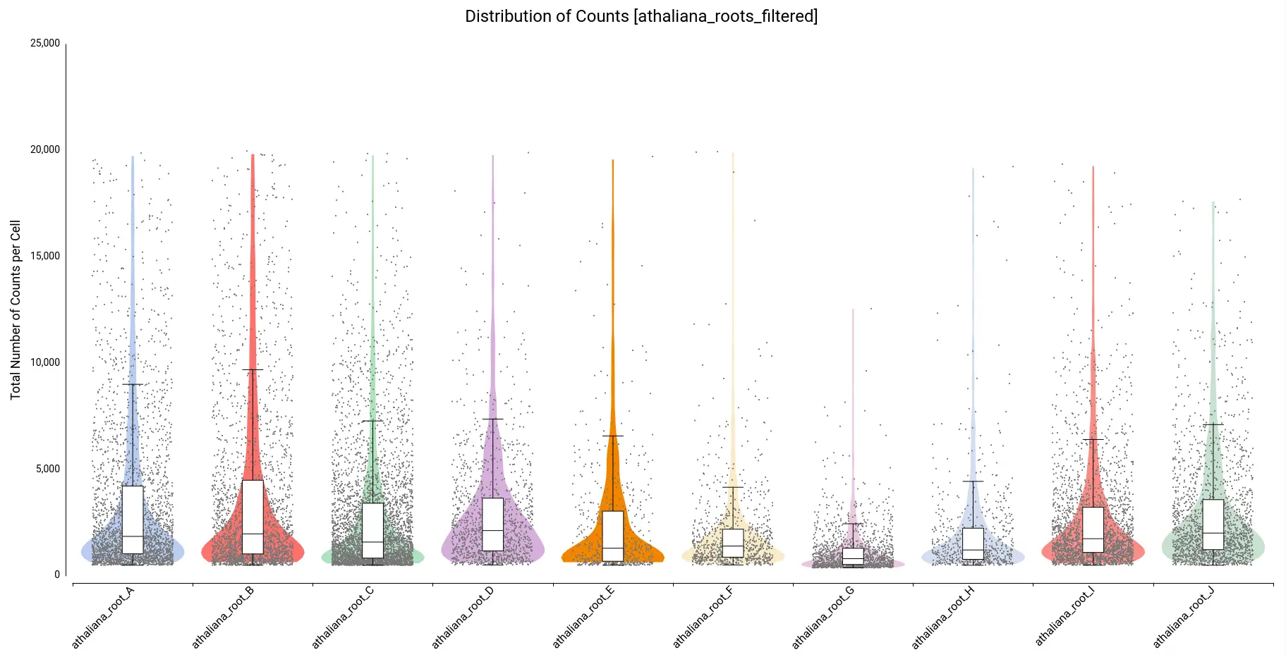
On the other hand, there are quite a number of cells with a comparatively higher number of counts. Thus, we decided to filter cells with a total number of counts greater than 20,000. Figure 6 shows the distribution after filtering.
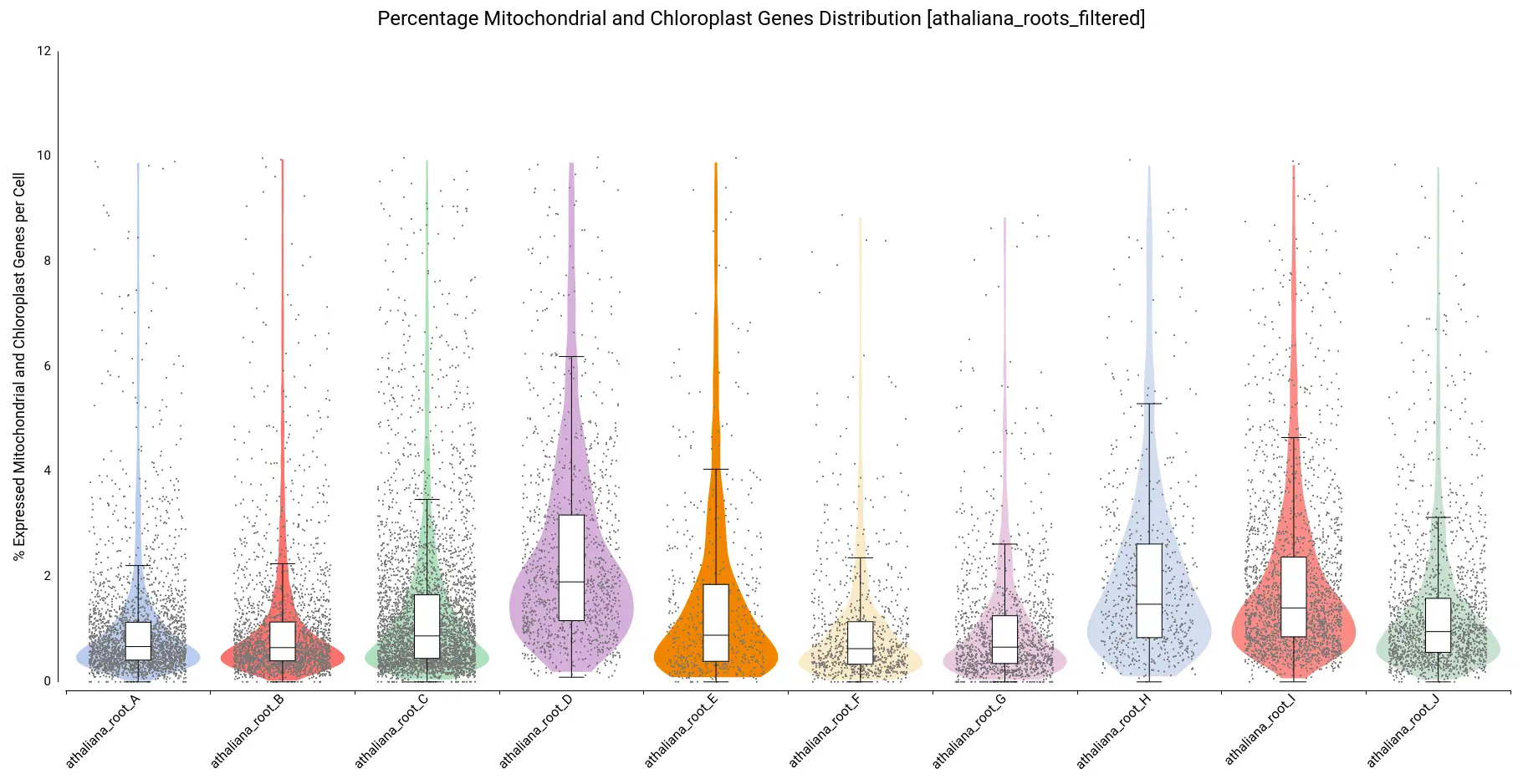
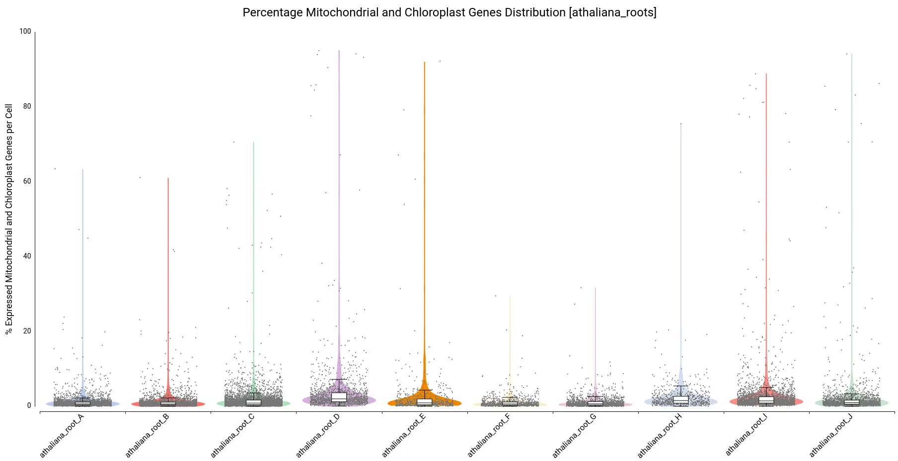
Moreover, violin and boxplots of the percentage of expressed genes belonging to mitochondria and chloroplast were also generated (Figure 7). Cells with a high percentage of those genes may be broken or dying cells, so it is recommended not to keep them for further analysis.
We filtered all cells with a percentage higher than 10, resulting in a count table with the distribution shown in Figure 8.
Finally, genes not expressed in a minimum of 100 cells were discarded, as well as cells not expressing a minimum of 200 genes. This is meant to reduce non-significant signals, as well as reduce the computational cost of downstream analysis.
💡 How to decide a filtering threshold
Violin and box plots aid in the threshold decision for filtering. The violin plot is more of a visual aid, whereas the box plot provides more precise statistical values. The width of the violin plot represents the density of cells in that particular area of the plot, so we could choose the point at which the violin shape narrows, since from this point cells could be considered outliers.
On the other hand, we could take the upper whisker value since points beyond this value are statistically defined as outliers. However, as we can see in Figure 9, this value is usually more stringent than the narrowing point of the violin plot.
Generally speaking, the threshold obtained with the violin plot is recommended and works well in most cases. The whisker threshold may be overly stringent, taking into account that single-cell data tend to be really sparse and a lot of cells will be lost due to low counts, and another bunch will be marked as poor-quality cells. Nevertheless, the boxplot still gives interesting metrics about the distribution like the median number of counts. In scenarios with an overall high number of counts, the whisker threshold may be appropriate as well.
scRNA-Seq Clustering
The Single-cell RNA-Seq clustering aims to identify groups of cells with similar expression patterns. These clusters can be further investigated in downstream analyses in order to elucidate different cell types, sub-cell types, cell states, study differences between conditions at the cell-type level, etc. Clusters are commonly the first piece of evidence of the single-cell analysis puzzle. However, raw counts, even after filtering, can’t be directly used for clustering. A typical scRNA-Seq pipeline consists of a list of preprocessing steps to prepare the data for clustering analysis, including normalization, dimensional reduction, data integration, etc. All these preprocessing steps, along with the clustering, were performed with the OmicsBox’ Seurat implementation.
Following the parameters used in the original paper (Shulse et al., 2019), we regressed out the variance due to the percent of mitochondria and chloroplast genes (“Data Correction” section). Additionally, we integrated the datasets by the “Medium” condition (Figure 3) using the Canonical Correlation Analysis (Seurat-CCA) method (Butler et al., 2018) using 35 dimensions. Finally, 20 dimensions were used for clustering, with a resolution of 0.6. The rest of the analysis parameters were left by default.
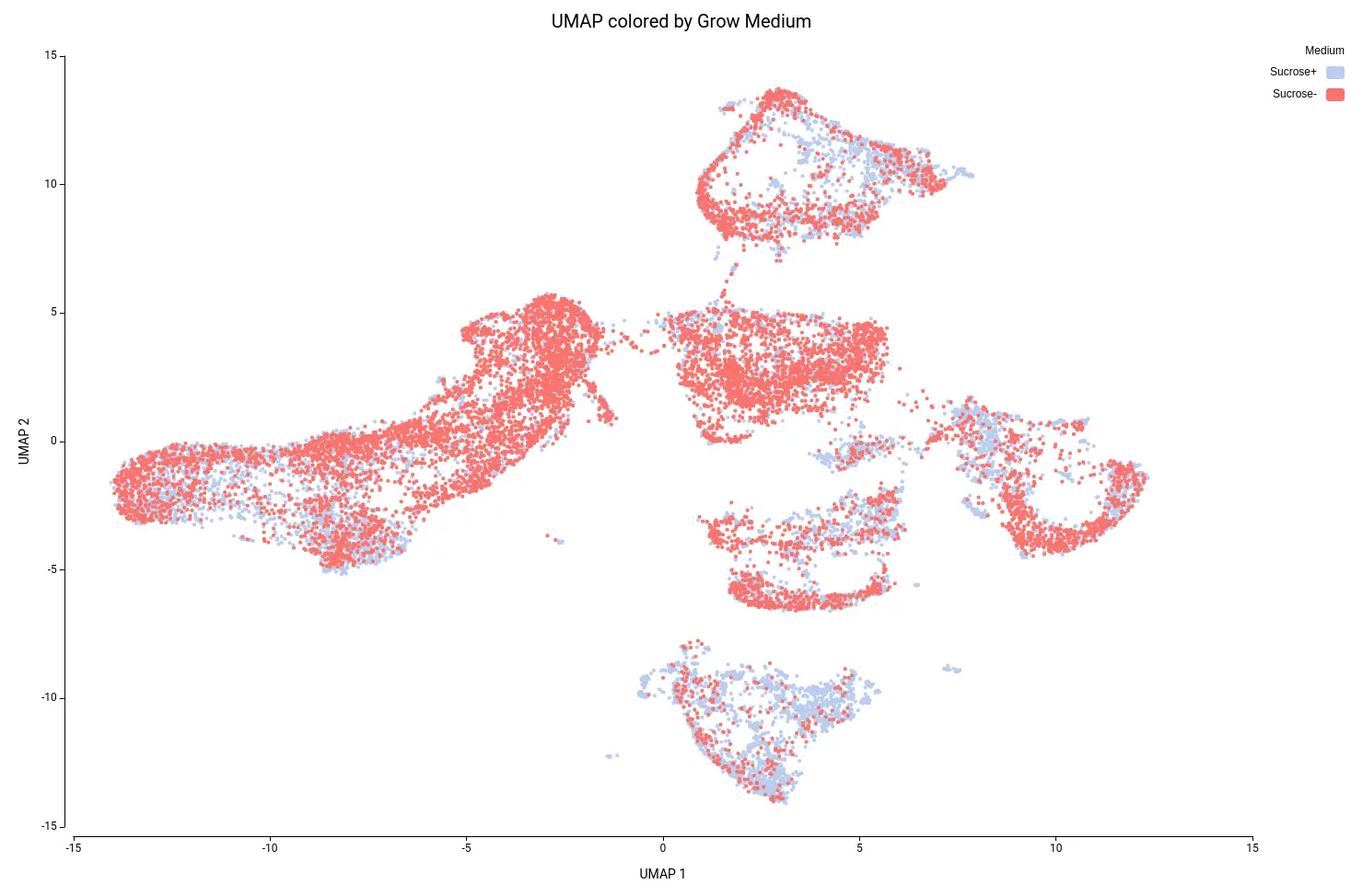
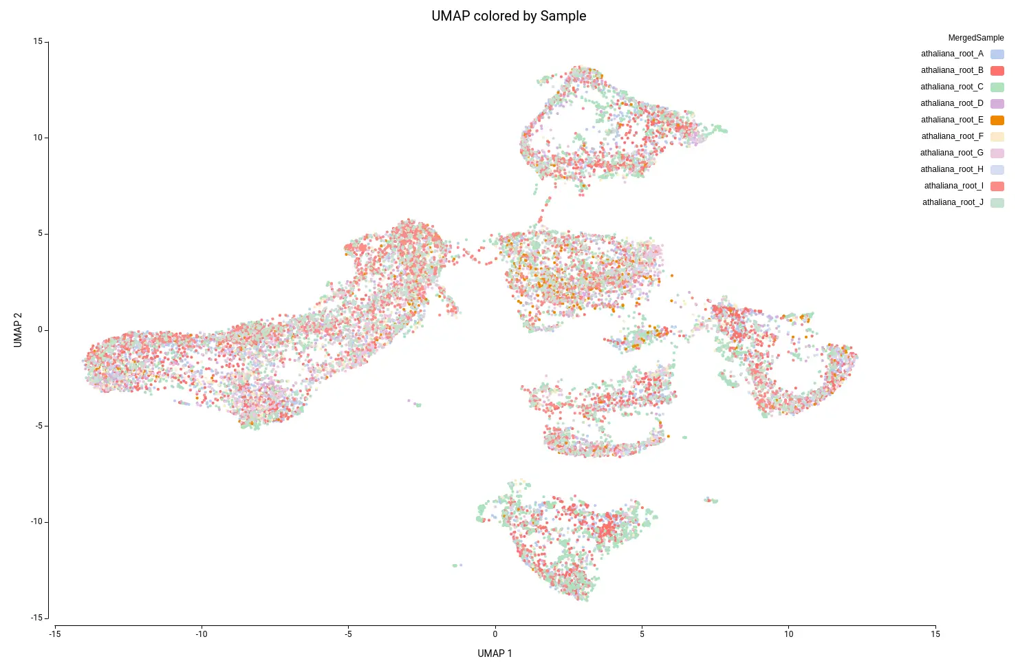
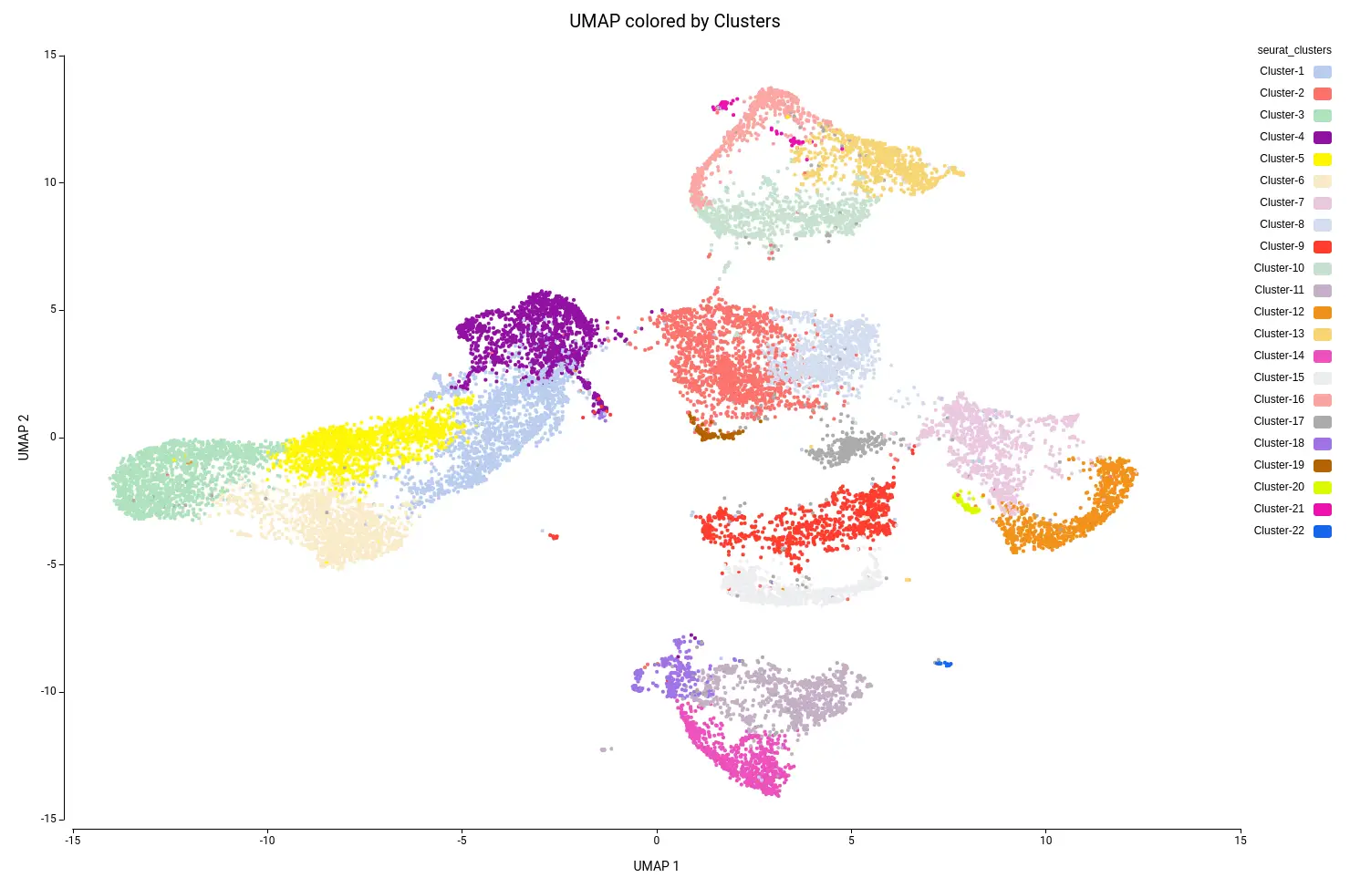
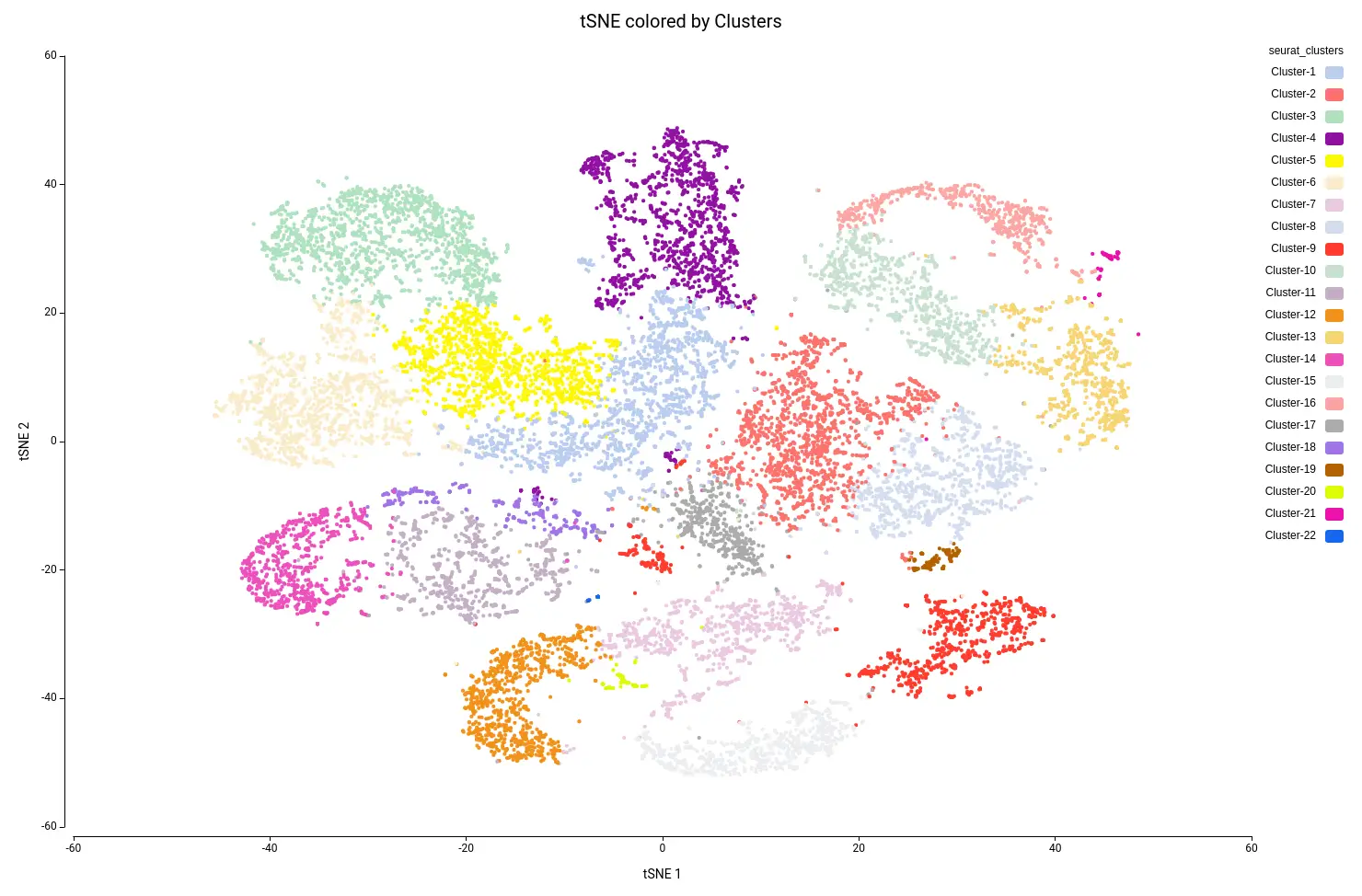
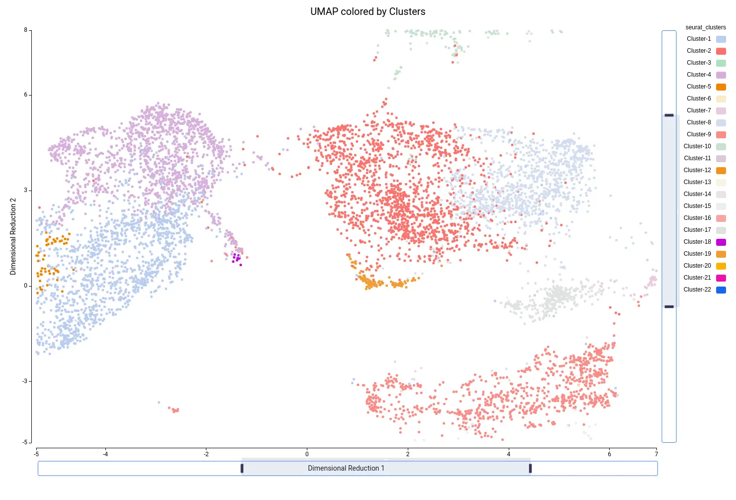
This analysis resulted in a total of 22 clusters (Figures 10 and 11), including cells from all grown mediums and samples (Figures 12 and 13). This shows that the integration has been successful and, thanks to it, cells with similar expression patterns have been detected in the two conditions. Nevertheless, it is noticeable that Clusters 11, 14, and 18 have a higher proportion of cells grown in medium with high sucrose (Figures 10 and 12). This is in concordance with the findings obtained in the original paper.
💡 How to decide a good number of dimensions (PCs)
Ideally, we would like to include a sufficient number of dimensions that effectively summarize all biological variance, but without adding uninteresting or noisy variance. On this matter, the Elbow Plot (Figure 14) helps identify a good number of dimensions. This plot shows the PCs (or dimensions) computed and their standard deviation, which is equivalent to the amount of variance explained by each of them.
By PCA definition, the amount of variability explained by successive PCs decreases, until a point in which successive PCs do not explain more variability. This is a good starting point for deciding the final number of dimensions to use. In Figure 14, this point will lay somewhere around 14 or 20 PCs.
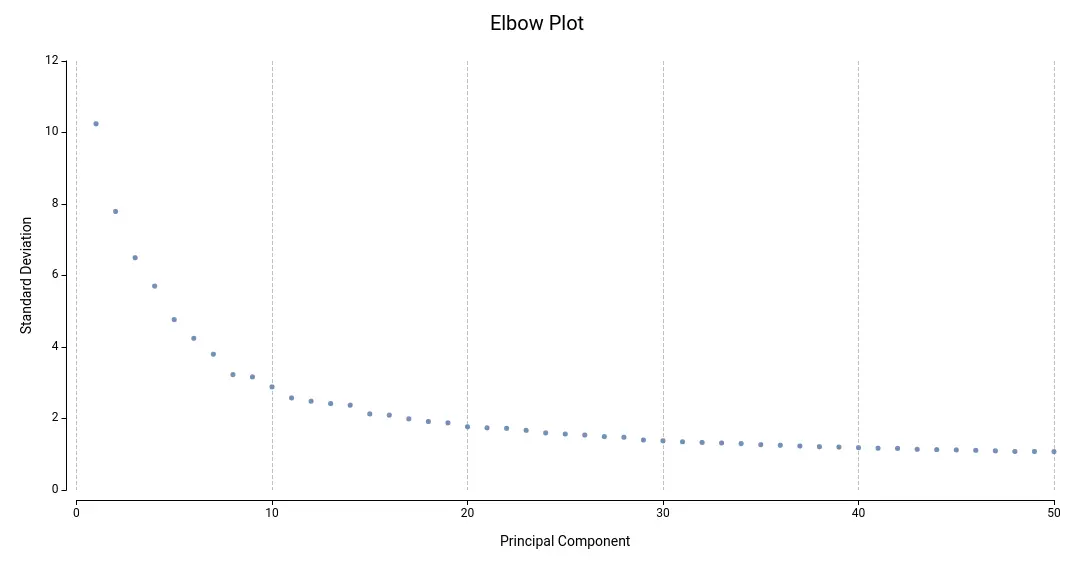
In general, it may be recommended to run the clustering with a different number of dimensions and assess the results. For example, if the resulting clustering contains a lot of small clusters, it is probable that they are not real cell types or states, but rather artifacts. Moreover, if we see that the obtained clusters are split into different areas of the UMAP or tSNE projections, it may be appropriate to re-run the clustering with different parameters.
Reference-based Cell Type Annotation
In the original paper, the researchers used marker gene expression as well as the Index of Cell Identity (ICI) scores to predict cell types. These approaches have some drawbacks in terms of the manual labor required and the difficulties of finding a good set of marker genes. Nowadays, reference-based methods are widely used and have proven their reliability (Abdelaal, T., et al., 2019 ; Ma, W., 2021). Additionally, more and more references are becoming available. All these features make reference-based approaches more appealing.
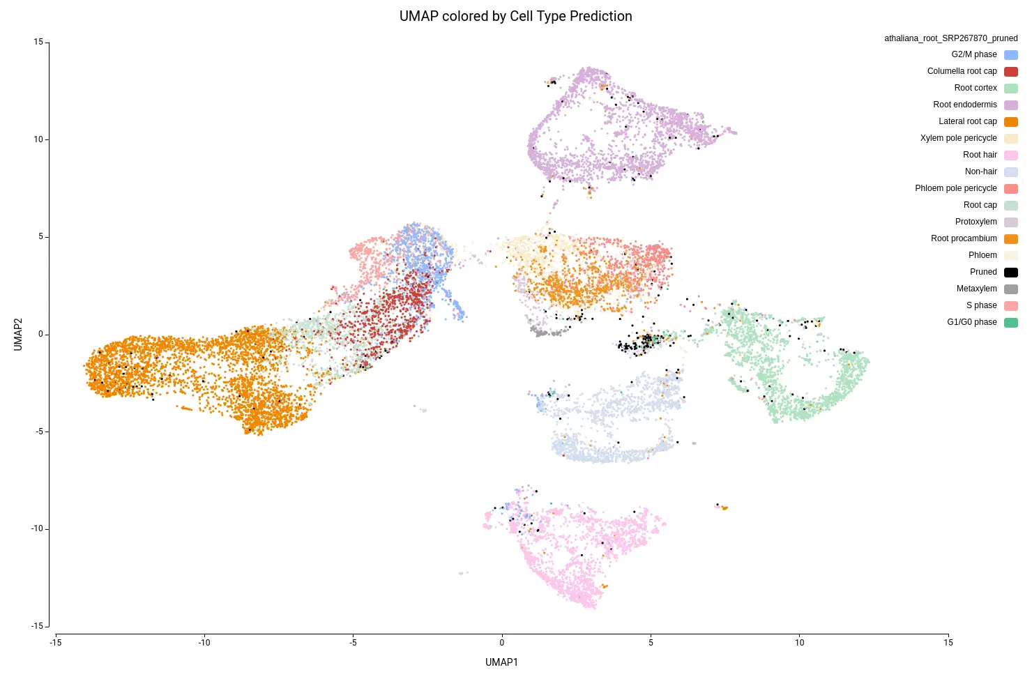
Thus, we used the SingleR OmicsBox implementation to perform the cell-type prediction. We downloaded a root tip Arabidopsis thaliana reference from the scPlantDB database, including 200K cells and 16 different cell types (SRP267870).
Figure 15 shows the UMAP projection with cells colored by the predicted cell types. We obtained 16 different cell type labels plus a “Pruned” category, which includes cells with an unreliable annotation, in contrast with the 7 general cell types detected in the original paper. These cells are mostly grouped in the same region as Cluster-17 (Figure 10), so this cluster is likely composed of poor-quality cells with misleading data or of cells of a cell type not present in the reference dataset.
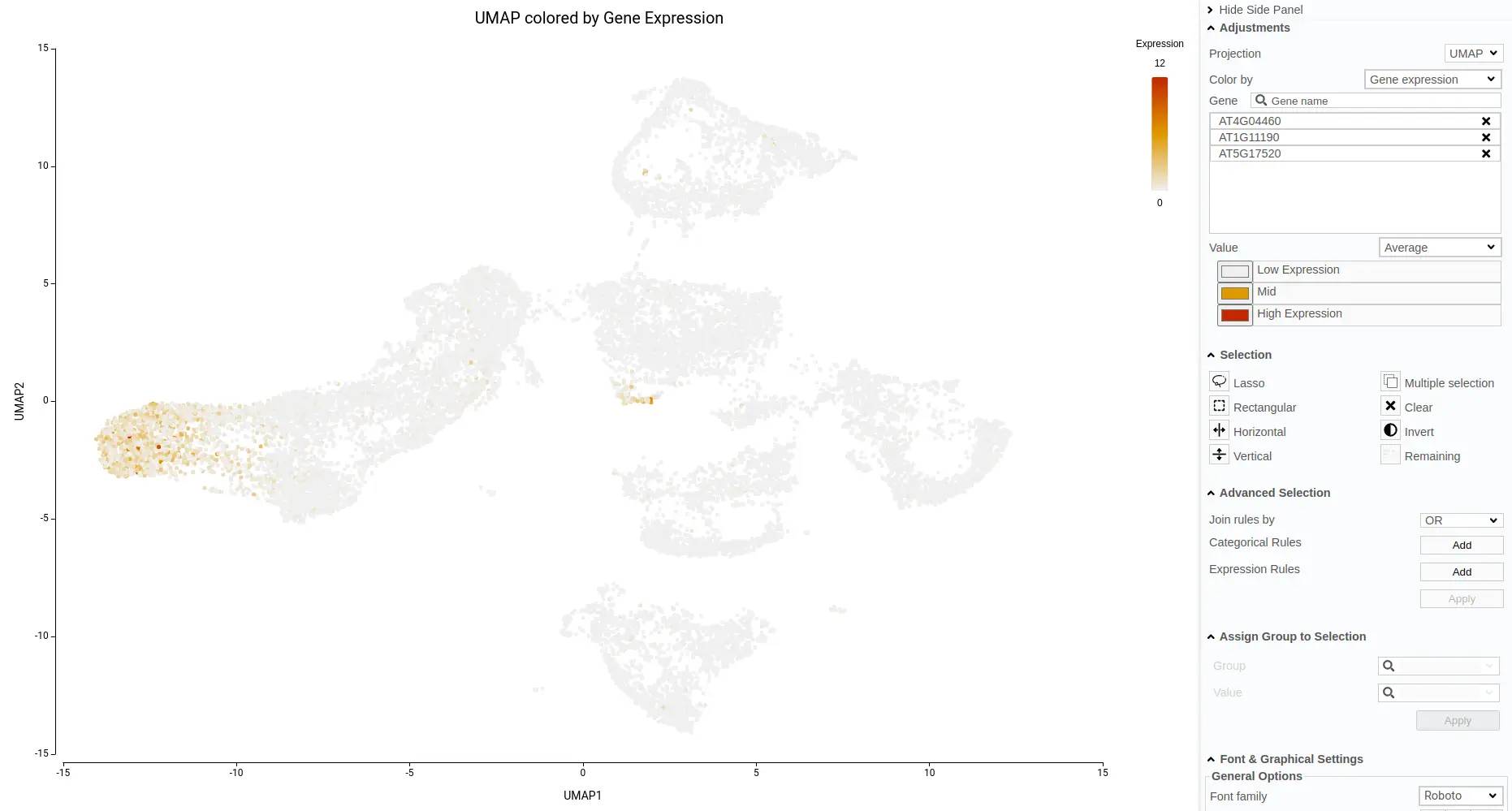
Another aspect to notice is that, in the original paper, they specifically stated that they were not able to identify the lateral root cap cells. However, with the reference-based annotation, it was possible to identify a large group of cells belonging to this cell type (Figure 15). This finding is further supported by a high expression of known lateral root cap marker genes in those cells (Figure 16).
💡 How to decide a good reference for cell-type prediction
The performance of the reference-based cell type annotation greatly depends on the reference dataset used. As general advice, the reference should be as similar as possible to the dataset being annotated: similar experimental procedures (e.g. cell extraction technique, growing conditions), obtained with the same library construction technology (e.g. 10x Chromium, Drop-seq), etc. Moreover, references consisting of multiple datasets tend to perform better.
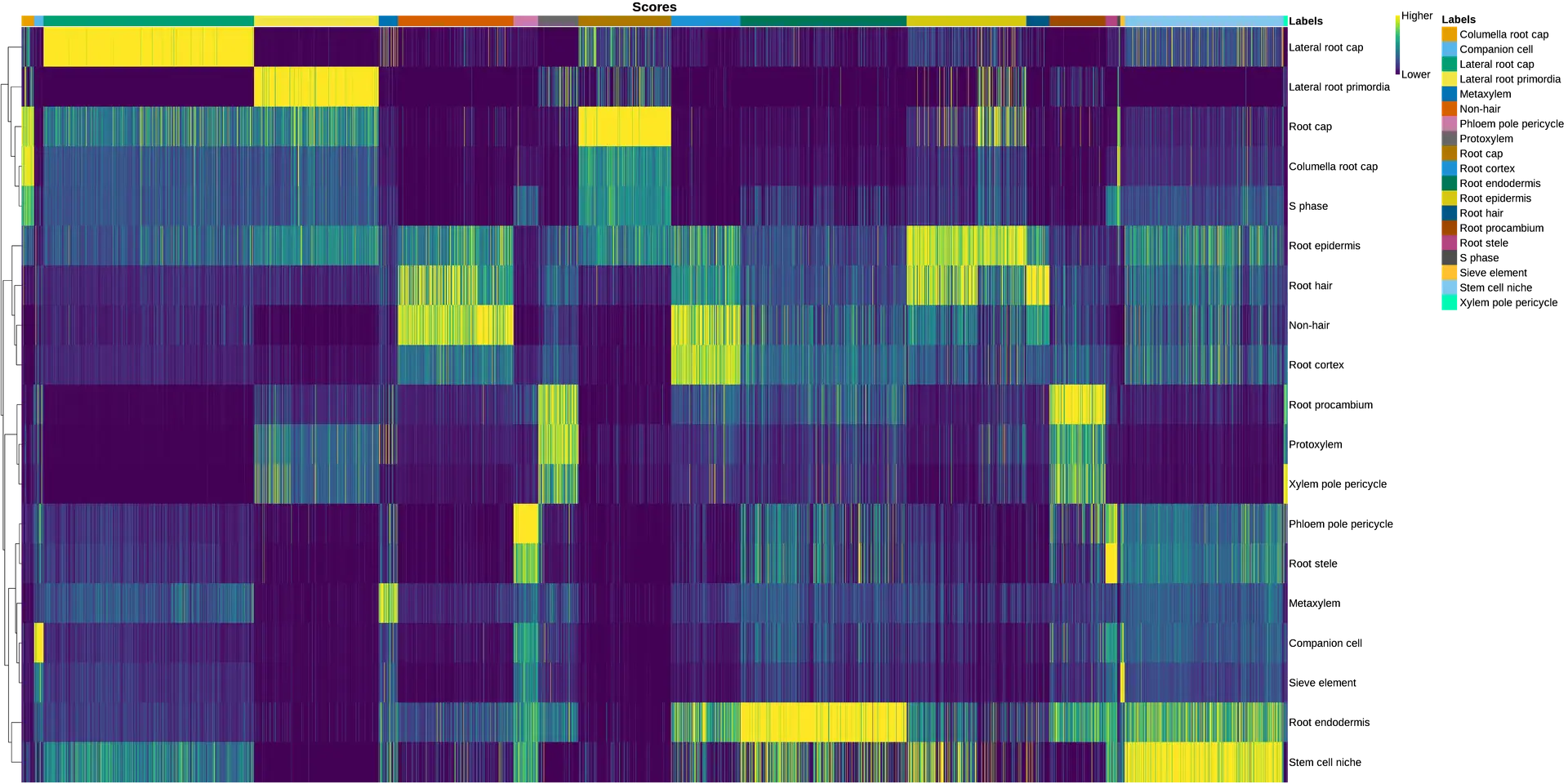
It is possible to assess how well a reference fits a dataset with the help of the SingleR’s heatmap and the UMAP visualization. In a perfect scenario, each cell in the dataset would have high prediction scores only for one cell type. However, a fuzzy heatmap like in Figure 17 means that each cell has multiple possible cell types, so the annotation is not that clean. This is also reflected in the UMAP visualization, where predicted cell types are dispersed in different areas and do not correspond to the obtained clusters (Figure 18).
Either way, it is recommended to perform various predictions with different references to establish a consensus.

Refining the Annotation
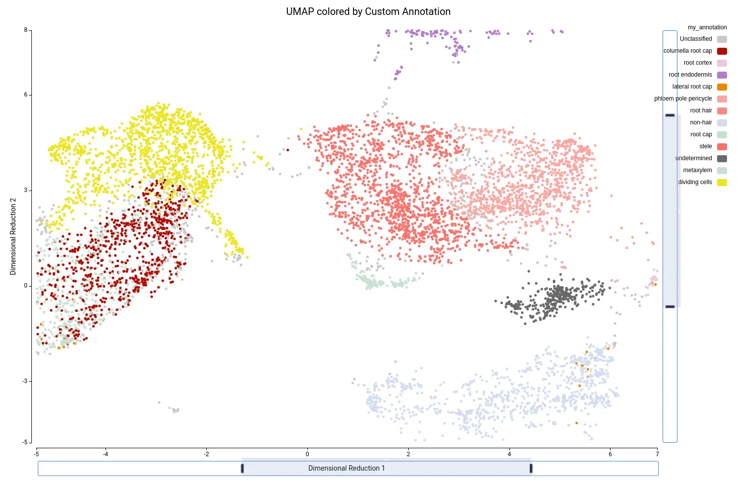
We combined the information obtained with the clustering and the cell type prediction in order to refine the annotation. The clustering tells us groups of similar cells in our particular dataset, whereas the cell type prediction tells us which cells are similar in the reference annotation. Using the UMAP/tSNE Viewer tools of the OmicsBox platform, we created our own custom annotation using these two pieces of evidence.
For example, if we zoom in on the central part of the UMAP, we see on the left part two precited cell types (“G2/M phase” and “S phase”, Figure 19) that are grouped into the same cluster (“Cluster-4”, Figure 20). Since we are not particularly interested in this division, we decided to group these cells into “Dividing cells” (Figure 21). Moreover, we see in the center that there are some cell type predictions mixed one with another (“Xylem pole pericicle”, “root procambium”, “protoxylem”, and “phloem”, Figure 19), which are grouped into the same cluster (“Cluster -2”, Figure 20). Since it is tricky to decide a clear border between these cell types we decided to group them into “Stele” cell type (Figure 21). We considered that this should require further analysis in order to clearly distinguish them. For example, by subsetting cells in Cluster-2 and running the clustering again. Finally, “Cluster-17” (Figure 20) is composed of many cell types (Figure 19) with an untrusting annotation (Figure 15), so we add those cells to a group named “undetermined” (Figure 21). This group should be further investigated as well to determine wether it could correspond to a cell type not present in the reference or to a spurious cluster. We continued this procedure with the rest of the cells, until reaching a complete custom annotation.

Differential Expression Analysis
Once cell groups are defined, whether they are clusters or cell types, the dataset can be interrogated with differential expression analysis. For example, we can test if there is any difference in gene expression between growing conditions (high sucrose and normal) in any cell type. We achieved it with the EdgeR implementation in OmicsBox, which is adapted to single-cell RNA-Seq data.
To follow the best single-cell differential expression practices, we further filtered lowly-expressed genes, by applying a threshold of 2 CPM in at least 200 cells.
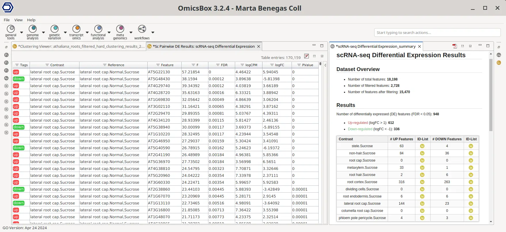
In addition, a pseudobulk analysis was performed by aggregating the cell counts of the same seedling (Figure 3) and cell type. Then, for each cell type, a differential expression test was performed between cells belonging to samples grown in a medium with high sucrose versus normal cells. This type of test is possible thanks to the data integration step performed during clustering (Figures 10 and 12). The test was easily configured with the OmicsBox graphical interface.
Figure 22 shows a summary table on the right with the number of differentially expressed genes (DEGs) for each test. For many cell types, none or very few DEGs were found, in concordance with the results obtained in the original paper. However, this is not the case for all cell types. For some of them, there were indeed some differences found between cell types.
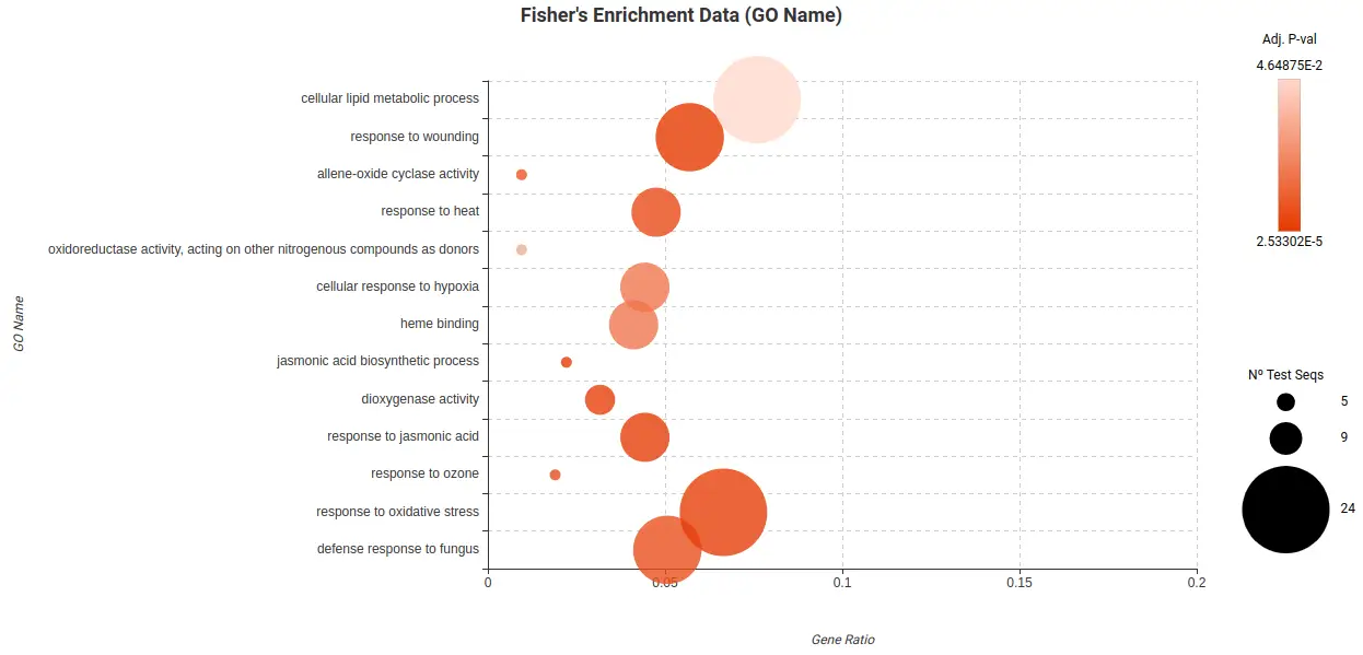
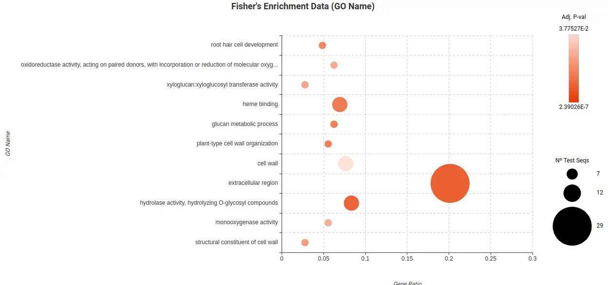
To further analyze and ease the interpretation of the DEGs lists obtained, a Fisher Exact Test (FET) was conducted to test if they were enriched in particular biological functions. In particular, there were enriched functions found in the Root Cortex (Figure 23) and Lateral Root Cap (Figure 24) related to response to stress, response to oxygen levels, and other biological process. These findings suggest that these cell types may indeed be affected by the high levels of sucrose present in the medium.
Conclusions
In this blog, we have seen how to perform a complete multi-sample single-cell RNA-Seq analysis pipeline for the plant Arabidopsis thaliana using OmicsBox. We started from raw reads and went through clustering and cell type prediction, down to biological interpretation of the results. Using the available tools, we have seen that mediums with high sucrose produce changes in the cell type composition and expression in the root tip.
References
- Shulse, C.N. et al. (2019). “High-throughput single-cell transcriptome profiling of plant cell types”. Cell Reports, 27(7). doi:10.1016/j.celrep.2019.04.054.
- Mortazavi, A., Williams, B., McCue, K. et al (2008). “Mapping and quantifying mammalian transcriptomes by RNA-Seq”. Nat Methods 5, 621–628. doi:10.1038/nmeth.1226
- Butler, Andrew et al. (2018). “Integrating single-cell transcriptomic data across different conditions, technologies, and species.” Nature biotechnology vol. 36,5 : 411-420. doi:10.1038/nbt.4096
- Abdelaal, T., Michielsen, L., Cats, D. et al. (2019). “A comparison of automatic cell identification methods for single-cell RNA sequencing data”. Genome Biol 20, 194. doi:10.1186/s13059-019-1795-z
- Ma, W., Su, K. and Wu, H. (2021). “Evaluation of some aspects in supervised cell type identification for single-cell RNA-seq: classifier, feature selection, and reference construction”. Genome Biol 22, 264. doi: 10.1186/s13059-021-02480-2
")