Comparing taxonomic and functional compositions in metagenomic samples

Any annotation of metagenomic sequences, whether it involves pathways, clusters of orthologous genes, species or any other taxonomic or functional classification can be compared across samples. These analyses are encompassed within the Differential Abundance Analysis, and they require robust statistical approaches to achieve reliable results because metagenomics datasets often show under-sampling and low signal-to-noise ratios.

All differential abundance analyses can be divided into three steps:

1. Functional Annotation or Taxonomic Classification.
2. Quantifying the abundance for each feature.
3. Evaluating the statistical significance with an appropriate test.

Differential Abundance Analysis aims at detecting differences in taxonomic or functional composition between metagenomic samples.

These kinds of tests have been studied extensively in other scenarios, concretely in differential expression studies of RNA-Seq data. The assumptions about the underlying distribution of counts of features are also applicable to Metagenomics datasets (e.g. Overdispersed Poisson or Negative Binomial).

In OmicsBox, two different Differential Abundance Analysis are available:

Differential Abundance Analysis of Taxa

The Differential Abundance Analysis of Taxa aims at detecting differences in taxonomic composition between samples or conditions. The results of this method are important in many fields in microbiology: in ecology, to detect differences between samples with different conditions; in medicine, to demonstrate the efficacy of antibiotic drugs; etc.

This analysis can be carried out easily in OmicsBox. First, a Kraken Taxonomic Classification project must be created. You can use our Taxonomic Classification tool or load a Kraken result via File > Load > Load Kraken Data.

Once loaded, the analysis can be executed under Metagenomics > Comparative Analysis > Differential Abundance Analysis of Taxas. The test can be configured easily: choose a proper method for filtering and normalization, select an experimental design, the taxonomic level, and a statistical test.

• Filtering. Taxas with low counts will not be considered for the test as they provide little evidence of differential abundance. There are two available filters: the Counts per Million Filter, to exclude taxas with low counts across all samples, and the Minimum Samples Filter, to exclude low abundance taxas in a minimum number of samples.
• Normalization. You can select correctional factors to scale the library sizes for all samples. There are four possible normalization methods, but TMMwsp (Trimmed Mean of M-values with singleton pairing) is recommended because performs better for data with a high proportion of zeros, which is common in metagenomic datasets.
• Experimental Design. Choose the contrast group and the reference group of samples. You can also include a pairing factor for experiments with block designs.
• Statistical Test. The statistical test can be selected. Basically, there are three different options: an exact test for pairwise comparisons and a negative binomial GLM with two different configurations (Likelihood Ratio Test and Quasi Likelihood F-Test, recommended for experiments with few replicates).

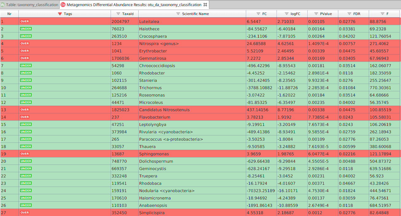
The main results are displayed in a table. Each row contains the tested taxa, and the different columns show:

• Taxonomic ID and scientific name.
• Tag. Indicates if the taxa is over or under-represented in the contrast group.
• Effect Size (Fold Change and Log Fold Change). The ratio between the abundance in the contrast condition and its abundance in the reference condition.
• Test Statistic of the statistical analysis. F-statistic or Likelihood Ratio (LR).
• Significance. P-value and FDR correction for multiple comparisons for the null hypothesis of non-differential abundance.

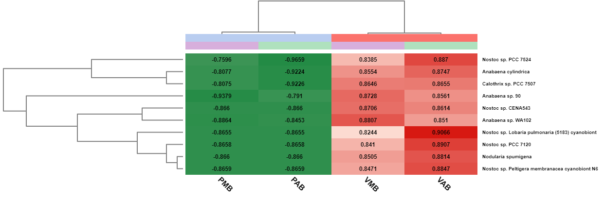
Furthermore, a summary report and a heatmap with a cluster analysis can be generated to visualize the results. This heatmap shows the relative abundance in each sample of the most abundant taxa. In addition, a hierarchical clustering of the samples and the taxa are displayed to see which features share a similar behaviour.

Differential Abundance Analysis of Functions

The Differential Abundance Analysis of Functions is designed to detect which functional annotations are differentially abundant between two conditions. The objective of this analysis is to compare two microbial communities at functional level (pathways, genes, protein domains, etc.).

In OmicsBox, this analysis compares the functional annotations between metagenomes of different samples, grouping them in two conditions. Several previous steps have to be carried out for each sample before the test: assembly (MEGAHIT or MetaSPAdes), gene prediction (FragGeneScan or Prodigal) and Functional Annotation (PfamScan or EggNOG-Mapper).

Once we have a functional annotation of each sample, run the test in Metagenomics > Comparative Analysis > Differential Abundance Analysis of Pfam / EggNOG. The different annotation objects have to be loaded and the test has to be configured: choose an adequate filter for poorly annotated features, set an experimental design and decide which kind of annotation should be tested.

• Annotation Files. Firstly, all annotation files have to be selected. These files must be of the same type, either Pfam or EggNOG.
• Filtering. Choose a filter to exclude annotations with low abundance across samples: this filter sets the minimum number a feature has to be annotated to be considered for the test.
• Annotations to Compare. You can compare at Domain and at Family level with PfamScan annotations; or at Metabolic Pathway and at COG level if working with EggNOG annotations.

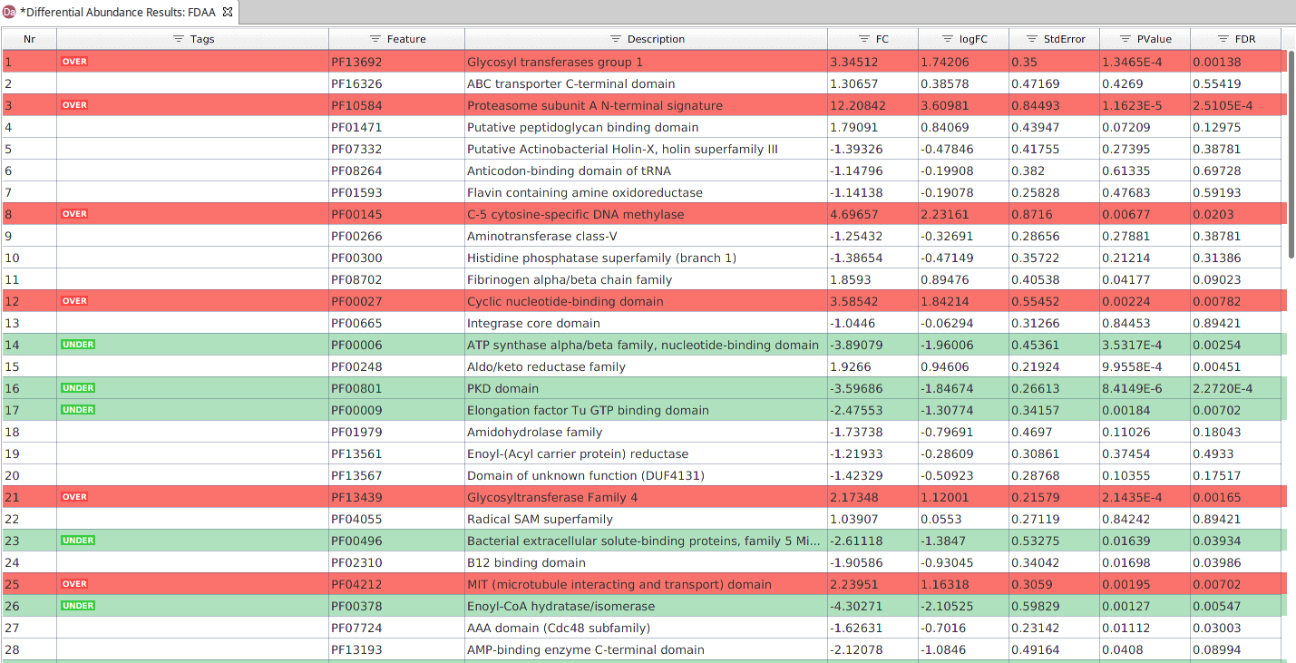
As in the previous test, the results are displayed in a table. In this case, each row contains an annotation and each column shows its:

• Feature and Description of the annotation.
• Tag. Indicates if the feature is over or under-represented in the contrast group.
• Effect Size (Fold Change and Log Fold Change).
• Standard Error of the estimation of the effect.
• Significance. P-value and FDR.

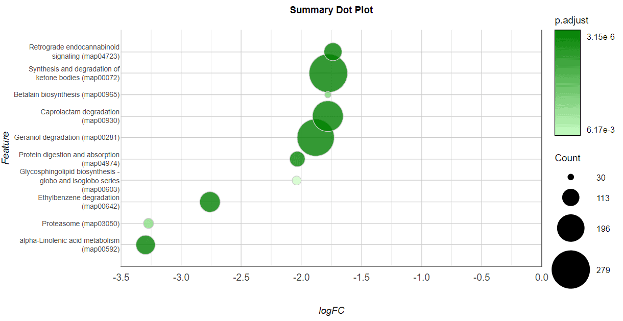
The results can be summarized in a Summary Dot Plot, a visually attractive graph which shows the features sorted by significance or by effect size. Each row of this plot contains a differentially abundant feature. The X-axis represents the effect size (logFC), the dot color represents the significance (FDR), and the dot size represents the number of genes in the global dataset annotated with this feature.

For further information, read the OmicsBox User Manual.

References

1. Luo, C., Rodriguez-R, L. M., & Konstantinidis, K. T. (2013). A User’s Guide to Quantitative and Comparative Analysis of Metagenomic Datasets. In Methods in Enzymology (pp. 525–547)
2. Weiss, S., Xu, Z.Z., Peddada, S. et al. Normalization and microbial differential abundance strategies depend upon data characteristics. Microbiome 5, 27 (2017)
3. Robinson MD, McCarthy DJ and Smyth GK (2010). “edgeR: a Bioconductor package for differential expression analysis of digital gene expression data.” Bioinformatics, 26